Zoom Julia basics
Zoom session 2 — part 2
Topic: In this lesson, we will cover the basics of Julia.
Variables
A variable is a name bound to a value:
a = 3Notice that, when you are in the REPL, Julia returns the value when you assign it to a variable. If you would like to prevent this, you need to add a semi-colon at the end of the expression:
b = "Hello, World!";To print a value in the REPL, you only need to call it:
a
If you want to print it while running a script however, you need to use the println() function:
println(a)You can reassign values to variables:
a = 3;
a = -8,2;
a
You can define multiple variables at once:
a, b, c = 1, 2, 3
b
Variables in Julia are case-sensitive and can include Unicode characters:
δ = 8.5;Built-in keywords are not allowed. Neither are built-in constants and keywords in use in a session.
false = 3;

> ERROR: syntax: invalid assignment location "false"
The keyword ans is a variable which, in the REPL, automatically takes the value of the last computed value:
a = 3
typeof(ans)
ans + 1

b = "test"
typeof(ans)
Unicode support
You can enter Unicode characters via tab completion of LaTeX abbreviations:
\omega		 # press TAB
\sum  		 # press TAB
\sqrt	     # press TAB
\in  	     # press TAB
\:phone :    # no space before colon (I added it to prevent parsing), press TAB
Comments
Comments do not get evaluated.
# Single line comment

#=
Comments can also spread over multiple lines
if you enclose them with this syntax
=#

x = 2;          # comments can be added at the end of lines
Data types
Type systems
Static type systems
In static type systems, the type of every expression is known and checked before the program is executed. This allows for faster execution of the program, but it is more constraining.
Examples of statically typed languages: C, C++, Java, Fortran, Haskell.
Dynamic type systems
In dynamic type systems, the type safety of the program is checked at runtime. This makes for more fluid, but slower and languages.
Examples of dynamically typed languages: Python, JavaScript, PHP, Ruby, Lisp.
Julia: dynamically typed with optional type declaration
You don't have to define the types:
typeof(2)
typeof(2.0)
typeof("Hello, World!")
typeof(true)
typeof((2, 4, 1.0, "test"))
You can however do so for clearer, faster, and more robust code:
function floatsum(a, b)
    (a + b)::Float64
end

floatsum(2.3, 1.0)
This passed the check.
floatsum(2, 4)

> ERROR: TypeError: in typeassert, expected Float64, got a value of type Int64
This did not…
Type declaration is not yet supported on global variables. So this only works in local contexts.
Types in Julia
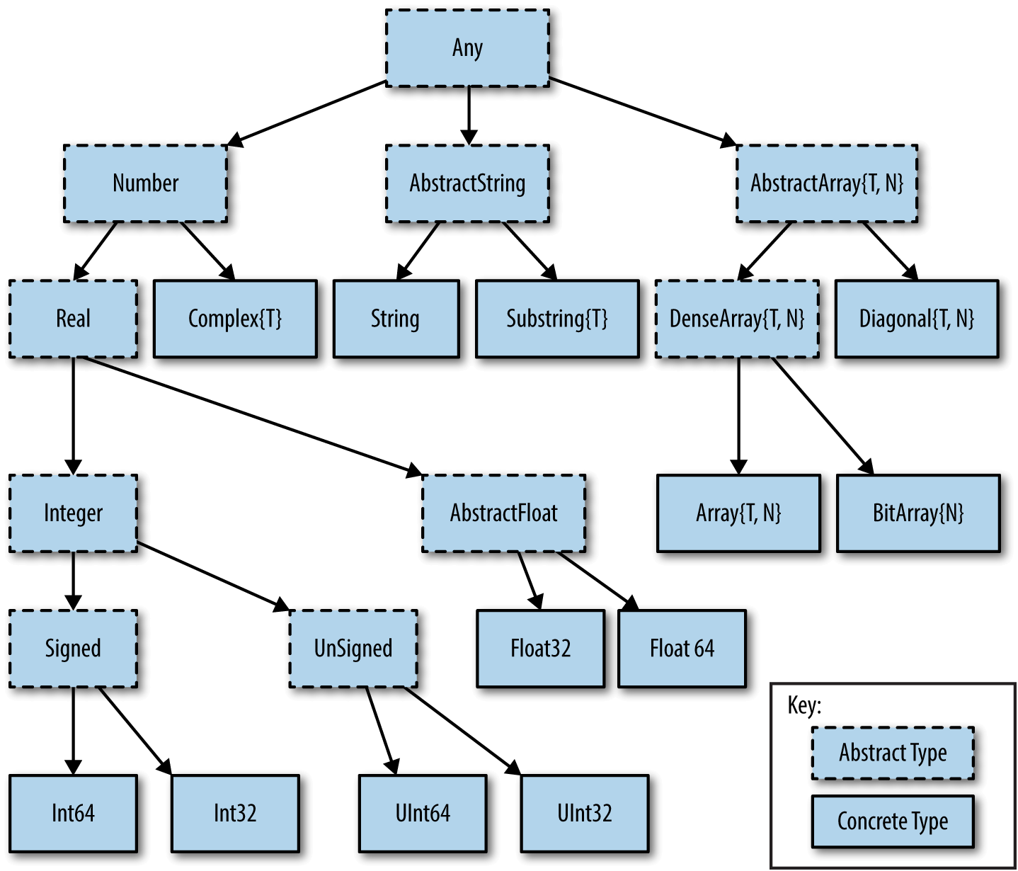
Julia's type system is much more elaborate than a collection of object implementations: it is a conceptual hierarchical tree, at the bottom of which are the concrete types. Above them are several levels of abstract types which only exist as concepts to allow for the construction of code suitable for a collection of concrete types. At the very top is the Any type, encompassing all types.
Quotes
Notice the difference between single and double quotes:
typeof("a")
typeof('a')

println("This is a string")
println('Ouch')

> ERROR: syntax: character literal contains multiple characters
Operators
The operators are functions. For instance, you can use the addition operator (+) in 2 ways:
3 + 2
+(3, 2)
The multiplication operator can be omitted when this does not create any ambiguity:
a = 3;
2a
Julia has "assignment by operation" operators:
a = 2;
a += 7    # this is the same as a = a + 7
There is a left division operator:
2\8 == 8/2The boolean type is a subtype of the integer type:
Bool <: Integer

false == 0
true == 1

a = true
b = false
3a + 2b
Julia supports fraction operations:
4//8
1//2 + 3//4
Collections of elements
Tuples
Immutable, indexable, possibly heterogeneous collections of elements:
typeof((2, 4, 1.0, "test"))
(2, 4, 1.0, "test")[2]
Named tuples
Tuples can have named components:
typeof((a=2, b=4, c=1.0, d="test"))

x = (a=2, b=4, c=1.0, d="test");
x[4] == x.d
Dictionaries
Similarly to Python, Julia has dictionaries: associative collections of key/value pairs:
Dict("a"=>1, "b"=>2, "c"=>3)Arrays
Arrays are mutable, indexable, homogeneous collections of elements.
One dimension
Unidimensional arrays of one element:
[3]
[3.4]
["Hello, World!"]
Unidimensional arrays of multiple elements:
[3, 4]Arrays are homogeneous collections, but look how Julia's abstract types make the following array possible:
[3, "hello"]These 4 syntaxes are equivalent:
[2
4
8]
[2; 4; 8]
vcat(2, 4, 8)
cat(2, 4, 8, dims=1)
Two dimensions
[3 4]
[[1, 3] [1, 2]]
These 3 syntaxes are equivalent:
[2 4 8]
hcat(2, 4, 8)
cat(2, 4, 8, dims=2)
Syntax subtleties
Elements separated by semi-colons or end of line get expanded vertically. Those separated by commas do not get expanded. Elements separated by spaces or tabs get expanded horizontally.
[1:2; 3:4]

[1:2
 3:4]

[1:2, 3:4]

[1:2 3:4]
Initializing arrays
Here are a few of the functions initializing arrays:
rand(2, 3, 4)
rand(Int64, 2, 3, 4)
zeros(Int64, 2, 5)
ones(2, 5)
reshape([1, 2, 4, 2], (2, 2))
fill("test", (2, 2))
Comprehensions
Julia has comprehensions similar to Python:
[ 3i + j for i=1:10, j=3 ]Indexing
As in other mathematically oriented languages such as R, Julia starts indexing at 1.
Indexing is done with square brackets:
a = [1 2; 3 4]
a[1, 1]
a[1, :]
a[:, 1]
b = ["wrong" "wrong" "wrong"; "wrong" "wrong" "wrong"; "wrong" "you got it" "wrong"]As in Python, by default, arrays are passed by sharing:
a = [1, 2, 3];
a[1] = 0;
a
This prevents the unwanted copying of arrays.
Functions
Function definition
There are 2 ways to define a new function:
Long form
function <name>(<arguments>)
    <body>
end
Example:
function hello()
    println("Hello")
end
Assignment form
<name>(<arguments>) = <body>Example:
hello() = println("Hello")
The function hello defined with this compact syntax is exactly the same as the one we defined above with the longer syntax.
Calling functions
You call a function by running it followed by parentheses:
hello()Arguments
Our function hello does not accept any argument:
hello("Paul")

> ERROR: MethodError: no method matching hello(::String)
To define a function which accepts arguments, we need to add them in the function definition.
So maybe we could do this?
function hello(name)
    println("Hello name")
end

hello("Paul")
Oops. Not quite… This function works but does not give the result we wanted.
Here, we need to use string interpolation with the $ character:
function hello(name)
    println("Hello $name")
end

hello("Paul")
We can also set default argument values: if no arguments are given, the function is evaluated with the defaults.
function hello(name = "you")
    println("Hello $name")
end

hello("Paul")
hello()
Here is another example:
function addTwo(a)
      a + 2
  end

addTwo(3)

# This can be written in a terse format with:
addtwo = a -> a + 2

# With default argument:
function addSomethingOrTwo(a, b = 2)
      a + b
  end

addSomethingOrTwo(3)
addSomethingOrTwo(3, 4)
Returning the result
The value of the last expression is automatically returned, so return is unnecessary unless you want to return something else.
Look at these 5 functions:
function test1(x, y)
    x + y
end

function test2(x, y)
    return x + y
end

function test3(x, y)
    x * y
end

function test4(x, y)
    x * y
    x + y
end

function test5(x, y)
    return x * y
    x + y
end
test1(1, 2)
test2(1, 2)
test3(1, 2)
test4(1, 2)
test5(1, 2)
Then run these expressions to see whether you got it right.
Anonymous functions
Anonymous functions are functions which aren't given a name:
function (<arguments>)
    <body>
end
And in compact form:
<arguments> -> <body>Example:
function (name)
    println("Hello $name")
end
Compact form:
name -> println("Hello $name")When would you want to use anonymous functions?
This is very useful for functional programming (when you apply a function—for instance map —to other functions to apply them in a vectorized manner which avoids repetitions).
Example:
map(name -> println("Hello $name"), ["Paul", "Lucie", "Sophie"]);Pipes
The Julia pipe looks like this: |>.
It redirects the output of the expression on the left as the input of the expression on the right.
The following 2 expressions are thus equivalent:
println("Hello")
"Hello" |> println
Quick test:
sqrt(2) == 2 |> sqrtFunction composition
This is done with the composition operator ∘ (in the REPL, type \circ
then press <tab>
).
The following 2 expressions are equivalent:
<function2>(<function1>(<arguments>))

(<function2> ∘ <function1>)(<arguments>)
Example:
exp(+(-3, 1))

(exp ∘ +)(-3, 1)
function!()
! used after a function name indicates that the function modifies its argument(s).
Example:
a = [-2, 3, -5]

sort(a)
a

sort!(a)
a
Broadcasting
To apply a function to each element of a collection rather than to the collection as a whole, Julia uses broadcasting.
a = [-3, 2, -5]
abs(a)

> ERROR: MethodError: no method matching abs(::Array{Int64,1})
This doesn't work because the function abs only applies to single elements.
By broadcasting abs, you apply it to each element of a:
broadcast(abs, a)The dot notation is equivalent:
abs.(a)It can also be applied to the pipe, to unary and binary operators, etc.
a .|> abs
abs.(a) == a .|> abs
abs.(a) .== a .|> abs
Methods
Julia uses multiple dispatch: functions can have several methods. When that is the case, the method applied depends on the types of all the arguments passed to the function (rather than only the first argument as is common in other languages).
methods(+)
let's you see that + has 166 methods!
Methods can be added to existing functions.
abssum(x::Int64, y::Int64) = abs(x + y)
abssum(x::Float64, y::Float64) = abs(x + y)

abssum(2, 4)
abssum(2.0, 4.0)
abssum(2, 4.0)
Control flow
Conditional statements
if
if <predicate>
    <do if true>
end
(If predicate evaluates to false, do nothing).
Example:
function testsign(x)
    if x >= 0
        println("x is positive")
    end
end

testsign(3)
testsign(0)
testsign(-2)
Predicates can be built with many operators and functions.
Examples of predicates:
occursin("that", "this and that")
4 < 3
a != b
2 in 1:3
3 <= 4 && 4 > 5
3 <= 4 || 4 > 5
if else
if <predicate>
    <do if true>
else
    <do if false>
end
Examples:
function testsign(x)
    if x >= 0
        println("x is positive")
    else
        println("x is negative")
    end
end

testsign(3)
testsign(0)
testsign(-2)
a = 2
b = 2.0
if a == b
println("It's true")
else
println("It's false")
end
if a === b
println("It's true")
else
println("It's false")
endThis can be written in a terse format:
<predicate> ? <do if true> : <do if false>Example:
a === b ? println("It's true") : println("It's false")if elseif else
if <predicate1>
    <do if predicate1 true>
elseif <predicate2>
    <do if predicate1 false and predicate2 true>
else
    <do if predicate1 and predicate2 false>
end
Example:
function testsign(x)
    if x > 0
        println("x is positive")
    elseif x == 0
        println("x is zero")
    else
        println("x is negative")
    end
end

testsign(3)
testsign(0)
testsign(-2)
Loops
while and for loops follow a syntax similar to that of functions:
for name = ["Paul", "Lucie", "Sophie"]
    println("Hello $name")
end
for i = 1:3, j = 3:5
println(i + j)
endi = 0
while i <= 10
println(i)
global i += 1
endMacros
Macros are a form of metaprogramming (the ability of a program to transform itself while running).
They resemble functions and just like functions, they accept as input a tuple of arguments. Unlike functions which return a value however, macros return an expression which is executed when the code is parsed (rather than at runtime). They are thus executed before the code is run.
Macro's names are preceded by @ (e.g. @time).
Julia comes with many macros and you can create your own with:
macro <name>()
    <body>
end
Sourcing a file
include() sources a Julia script:
include("/path/to/file.jl")